03 Data Science

# pip install pandas

# pip install matplotlib

# pip install seaborn

Series

import pandas as pd
import numpy as np
import matplotlib.pyplot as plt

import pandas as pd
series = pd.Series(["A","B","AB","O"])
series[4] = "O-"
print(series)

   A
   B
  AB
   O
  O-
dtype: object

series

   A
   B
  AB
   O
  O-
dtype: object

DataFrame

import pandas as pd
pd.__version__

'2.2.0'

import pandas as pd
data  = [1,2,3,4,5]
df1 = pd.DataFrame(data)
# display(df1)

data = [['Alice', 21], ['Bob', 22], ['Cathy', 23]]
df2 = pd.DataFrame(data, columns = ["Name", "Age"])
df2

	Name	Age
0	Alice	21
1	Bob	22
2	Cathy	23

d = {'name' : pd.Series(['Alice','Bob','Cathy','Dave']),
    'Age': pd.Series([21,22,23,24]),
    'Score' : pd.Series([80,85,90,95])}

df3 = pd.DataFrame(d)
df3

	name	Age	Score
0	Alice	21	80
1	Bob	22	85
2	Cathy	23	90
3	Dave	24	95

df3.info()

<class 'pandas.core.frame.DataFrame'>
RangeIndex: 4 entries, 0 to 3
Data columns (total 3 columns):
 #   Column  Non-Null Count  Dtype 
---  ------  --------------  ----- 
 0   name    4 non-null      object
 1   Age     4 non-null      int64 
 2   Score   4 non-null      int64 
dtypes: int64(2), object(1)
memory usage: 228.0+ bytes

df3.columns

Index(['name', 'Age', 'Score'], dtype='object')

for i in df3['name']:
    print(i)

Alice
Bob
Cathy
Dave

for i in df3['Age']:
    print(i)

df3

	name	Age	Score
0	Alice	21	80
1	Bob	22	85
2	Cathy	23	90
3	Dave	24	95

df4 = df3[df3['Score'] > 80]
df4

	name	Age	Score
1	Bob	22	85
2	Cathy	23	90
3	Dave	24	95

import pandas as pd
import matplotlib.pyplot as plt
import seaborn as sns

df = pd.read_csv('https://nontapatnon.github.io/python-course-master/datascience/Titanic-Dataset.csv')
df.head()

	PassengerId	Survived	Pclass	Name	Sex	Age	SibSp	Ticket	Fare	Cabin	Embarked
0	1	0	3	Braund, Mr. Owen Harris	male	22.0	1	A/5 21171	7.2500	NaN	S
1	2	1	1	Cumings, Mrs. John Bradley (Florence Briggs Th...	female	38.0	1	PC 17599	71.2833	C85	C
2	3	1	3	Heikkinen, Miss. Laina	female	26.0	0	STON/O2. 3101282	7.9250	NaN	S
3	4	1	1	Futrelle, Mrs. Jacques Heath (Lily May Peel)	female	35.0	1	113803	53.1000	C123	S
4	5	0	3	Allen, Mr. William Henry	male	35.0	0	373450	8.0500	NaN	S

df.info()

<class 'pandas.core.frame.DataFrame'>
RangeIndex: 891 entries, 0 to 890
Data columns (total 12 columns):
 #   Column       Non-Null Count  Dtype  
---  ------       --------------  -----  
 0   PassengerId  891 non-null    int64  
 1   Survived     891 non-null    int64  
 2   Pclass       891 non-null    int64  
 3   Name         891 non-null    object 
 4   Sex          891 non-null    object 
 5   Age          714 non-null    float64
 6   SibSp        891 non-null    int64  
 7   Parch        891 non-null    int64  
 8   Ticket       891 non-null    object 
 9   Fare         891 non-null    float64
 10  Cabin        204 non-null    object 
 11  Embarked     889 non-null    object 
dtypes: float64(2), int64(5), object(5)
memory usage: 83.7+ KB

df.columns

Index(['PassengerId', 'Survived', 'Pclass', 'Name', 'Sex', 'Age', 'SibSp',
       'Parch', 'Ticket', 'Fare', 'Cabin', 'Embarked'],
      dtype='object')

df[df['Survived'] == 0][['Name', 'Sex']]

	Name	Sex
0	Braund, Mr. Owen Harris	male
4	Allen, Mr. William Henry	male
5	Moran, Mr. James	male
6	McCarthy, Mr. Timothy J	male
7	Palsson, Master. Gosta Leonard	male
...	...	...
884	Sutehall, Mr. Henry Jr	male
885	Rice, Mrs. William (Margaret Norton)	female
886	Montvila, Rev. Juozas	male
888	Johnston, Miss. Catherine Helen "Carrie"	female
890	Dooley, Mr. Patrick	male

549 rows × 2 columns

df.head()

	PassengerId	Survived	Pclass	Name	Sex	Age	SibSp	Ticket	Fare	Cabin	Embarked
0	1	0	3	Braund, Mr. Owen Harris	male	22.0	1	A/5 21171	7.2500	NaN	S
1	2	1	1	Cumings, Mrs. John Bradley (Florence Briggs Th...	female	38.0	1	PC 17599	71.2833	C85	C
2	3	1	3	Heikkinen, Miss. Laina	female	26.0	0	STON/O2. 3101282	7.9250	NaN	S
3	4	1	1	Futrelle, Mrs. Jacques Heath (Lily May Peel)	female	35.0	1	113803	53.1000	C123	S
4	5	0	3	Allen, Mr. William Henry	male	35.0	0	373450	8.0500	NaN	S

df.head(10)

	PassengerId	Survived	Pclass	Name	Sex	Age	SibSp	Parch	Ticket	Fare	Cabin	Embarked
0	1	0	3	Braund, Mr. Owen Harris	male	22.0	1	0	A/5 21171	7.2500	NaN	S
1	2	1	1	Cumings, Mrs. John Bradley (Florence Briggs Th...	female	38.0	1	0	PC 17599	71.2833	C85	C
2	3	1	3	Heikkinen, Miss. Laina	female	26.0	0	0	STON/O2. 3101282	7.9250	NaN	S
3	4	1	1	Futrelle, Mrs. Jacques Heath (Lily May Peel)	female	35.0	1	0	113803	53.1000	C123	S
4	5	0	3	Allen, Mr. William Henry	male	35.0	0	0	373450	8.0500	NaN	S
5	6	0	3	Moran, Mr. James	male	NaN	0	0	330877	8.4583	NaN	Q
6	7	0	1	McCarthy, Mr. Timothy J	male	54.0	0	0	17463	51.8625	E46	S
7	8	0	3	Palsson, Master. Gosta Leonard	male	2.0	3	1	349909	21.0750	NaN	S
8	9	1	3	Johnson, Mrs. Oscar W (Elisabeth Vilhelmina Berg)	female	27.0	0	2	347742	11.1333	NaN	S
9	10	1	2	Nasser, Mrs. Nicholas (Adele Achem)	female	14.0	1	0	237736	30.0708	NaN	C

df.tail()

	PassengerId	Survived	Pclass	Name	Sex	Age	SibSp	Parch	Ticket	Fare	Cabin	Embarked
886	887	0	2	Montvila, Rev. Juozas	male	27.0	0	0	211536	13.00	NaN	S
887	888	1	1	Graham, Miss. Margaret Edith	female	19.0	0	0	112053	30.00	B42	S
888	889	0	3	Johnston, Miss. Catherine Helen "Carrie"	female	NaN	1	2	W./C. 6607	23.45	NaN	S
889	890	1	1	Behr, Mr. Karl Howell	male	26.0	0	0	111369	30.00	C148	C
890	891	0	3	Dooley, Mr. Patrick	male	32.0	0	0	370376	7.75	NaN	Q

import matplotlib.pyplot as plt
df['Survived'].value_counts()

Survived
0    549
1    342
Name: count, dtype: int64

df.groupby(['Sex','Survived'])[['Survived']].count()

		Survived
Sex	Survived
female	0	81
female	1	233
male	0	468
male	1	109

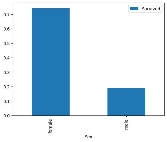
df[['Sex', 'Survived']].groupby(['Sex']).mean().plot.bar()
plt.show()

png

import matplotlib.pyplot as plt
import seaborn as sns

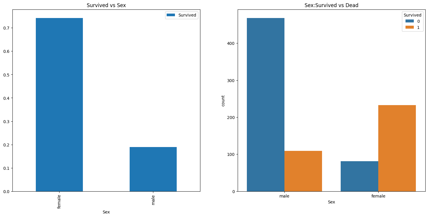
f, ax = plt.subplots(1, 2, figsize = (18,8))
ax[0].set_title('Survived vs Sex')
df[['Sex', 'Survived']].groupby(['Sex']).mean().plot.bar(ax = ax[0])

ax[1].set_title('Sex:Survived vs Dead')
sns.countplot(x = 'Sex', hue = 'Survived', data = df, ax = ax[1])
plt.show()

png

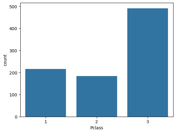
sns.countplot(df, x="Pclass")

<Axes: xlabel='Pclass', ylabel='count'>

png

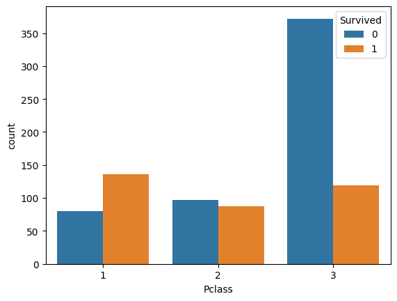
sns.countplot(data = df, x="Pclass", hue="Survived")

<Axes: xlabel='Pclass', ylabel='count'>

png

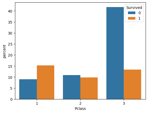
sns.countplot(data = df , x="Pclass", hue="Survived", stat="percent")

<Axes: xlabel='Pclass', ylabel='percent'>

png

Time Series Data

df_f = pd.read_csv("https://nontapatnon.github.io/python-course-master/datascience/flight2.csv")
df_f

	year	month	passengers
0	1949	Jan	112
1	1949	Feb	118
2	1949	Mar	132
3	1949	Apr	129
4	1949	May	121
...	...	...	...
139	1960	Aug	606
140	1960	Sep	508
141	1960	Oct	461
142	1960	Nov	390
143	1960	Dec	432

144 rows × 3 columns

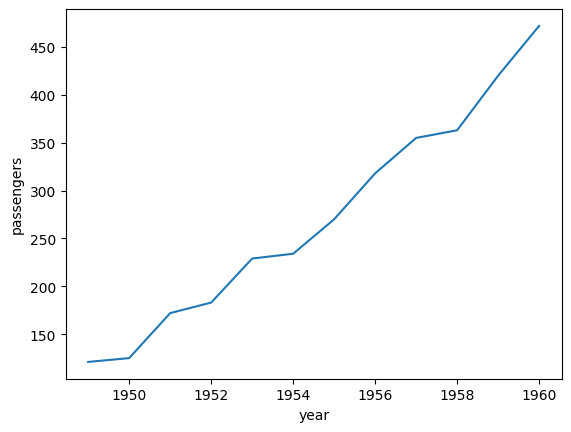
df_may = df_f.query("month == 'May'")
sns.lineplot(data = df_may, x = "year", y = "passengers")

<Axes: xlabel='year', ylabel='passengers'>

png

df_wide = df_f.pivot(index = "year", columns = "month", values= "passengers")
df_wide.head()

month	Apr	Aug	Dec	Feb	Jan	Jul	Jun	Mar	May	Nov	Oct	Sep
year
1949	129	148	118	118	112	148	135	132	121	104	119	136
1950	135	170	140	126	115	170	149	141	125	114	133	158
1951	163	199	166	150	145	199	178	178	172	146	162	184
1952	181	242	194	180	171	230	218	193	183	172	191	209
1953	235	272	201	196	196	264	243	236	229	180	211	237

sns.lineplot(data= df_wide["May"])

<Axes: xlabel='year', ylabel='May'>

png

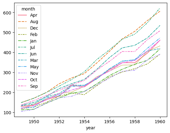
sns.lineplot(data = df_wide)

<Axes: xlabel='year'>

png

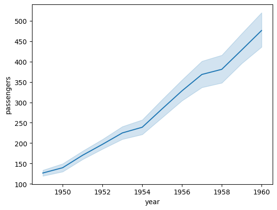
sns.lineplot(data=df_f, x="year", y="passengers")

<Axes: xlabel='year', ylabel='passengers'>

png

# pip install plotly

import plotly.express as px
import plotly.io as pio
pio.renderers.default = 'iframe'

df = px.data.iris()
df.head()

	sepal_length	sepal_width	petal_length	petal_width	species	species_id
0	5.1	3.5	1.4	0.2	setosa	1
1	4.9	3.0	1.4	0.2	setosa	1
2	4.7	3.2	1.3	0.2	setosa	1
3	4.6	3.1	1.5	0.2	setosa	1
4	5.0	3.6	1.4	0.2	setosa	1

fig = px.scatter(df, x="sepal_width", y="sepal_length", color="species",
                 size='petal_length', hover_data=['petal_width'])
fig.show()

import plotly.express as px
df = px.data.tips()
df.head()

	total_bill	tip	sex	smoker	day	time	size
0	16.99	1.01	Female	No	Sun	Dinner	2
1	10.34	1.66	Male	No	Sun	Dinner	3
2	21.01	3.50	Male	No	Sun	Dinner	3
3	23.68	3.31	Male	No	Sun	Dinner	2
4	24.59	3.61	Female	No	Sun	Dinner	4

df

	total_bill	tip	sex	smoker	day	time	size
0	16.99	1.01	Female	No	Sun	Dinner	2
1	10.34	1.66	Male	No	Sun	Dinner	3
2	21.01	3.50	Male	No	Sun	Dinner	3
3	23.68	3.31	Male	No	Sun	Dinner	2
4	24.59	3.61	Female	No	Sun	Dinner	4
...	...	...	...	...	...	...	...
239	29.03	5.92	Male	No	Sat	Dinner	3
240	27.18	2.00	Female	Yes	Sat	Dinner	2
241	22.67	2.00	Male	Yes	Sat	Dinner	2
242	17.82	1.75	Male	No	Sat	Dinner	2
243	18.78	3.00	Female	No	Thur	Dinner	2

244 rows × 7 columns

import plotly.express as px
df = px.data.tips()

fig = px.density_heatmap(df, x="total_bill", y="tip", text_auto=True)
fig.show()

Python Course Nontapat Thaiprayoon

03 Data Science

Series

DataFrame

Time Series Data